
with articles on technical aspects of photography.
|
Image Stabilization Measuring the Benefits |

|
Back to the Nitty-Gritty section, with articles on technical aspects of photography. |
|
Here I'm presenting a procedure which can be used to measure image stabilization benefits in picture-taking, and which I've been using in tests described on this site. For a general introduction to camera shake and image stabilization issues, refer to a separate article. |
|
Before you've invested your precious time into reading this article, this is the last warning: if you are looking for a procedure to provide a simple answer: "this IS system gives you 2 stops of advantage, compared to camera's A 1.5 stops and Camera's B 3 stops", stop reading and look elsewhere. If you decide to stay, be prepared to see some minutiae. I'm going to describe the whole process in detail, so that no part is hidden under a "trust me" cover. Choosing the right metrics Assuming all conditions (except for the controlled variables: shutter speed and IS status) remain unchanged over the whole experiment, every time we take a picture, there is some probability of it coming acceptably sharp. This probability depends on the control variables, and, for obvious reasons, its values will be close to zero at low shutter speeds, approaching 100% at speeds high enough.
Mind it, this is just an illustration, as we do not know the exact shape of such a dependency; we can only try to approximate it using experimental methods, based on a large population of trials. Let us assume for a while, that we have done that already, just to see how we could then define a metrics describing the benefits of using the IS in our camera.
Figure 1 shows two such dependencies; one
with image stabilization (green) and one without (yellow). The probability of success (i.e., obtaining a picture without motion blur) is shown on the y-axis, while the x-axis shows the shutter speed in terms of EV stops from our chosen base value of 1s.
| In all our calculations we will call this variable v and define it as v=log2s, where s is the shutter speed denominator (in seconds). In other words, v is the EV offset from a shutter speed of 1 s. For example, if the shutter speed is 1/8 s, the value of v will be log28 which is 3.
| 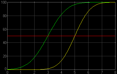
| Figure 1. The success (no blur) probability versus shutter speed (EV) at a given focal length, all other factors equal, with and without IS.
| With image stabilization we can shoot, on average, at slower shutter speeds (lower EV), achieving the same results (in terms of camera-shake blur) as at higher speeds without IS: the green line runs to the left of the yellow one. The horizontal offset between the lines could be a good measure of the benefits of image stabilization. The problem is that this distance may (and usually does) change with the probability level. (In this example the lines run closer at the top than at the bottom.) For a number of reasons I prefer to measure that distance at the level of a 50% success rate, marked with the red line. This is reasonable and leaves least room for misuse, also being statistically most robust, not based on tails of distributions. Therefore: For the metrics describing benefits of image stabilization at a given focal length we will choose the difference between a shutter speed providing a 50% success rate without IS and such speed with IS.
This corresponds to the distance between yellow/red and green/red intersection points in In this example the green (IS) line crosses the 50% level at v50=3 EV (1/8 s); for the yellow (no IS) one v50=5 EV (1/32 s). The difference between the two is Δv50=2 EV, which means shutter speeds longer by a factor of 4×. Benefit metrics estimation
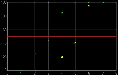
Things would be just peachy, then, if we only had the data for two lines shown in To do that, we can use some discrete EV values (shutter speeds), for each taking a number of pictures, and see what percentage is free of blur. The more frames we add to the statistics, the better will our points represent the real probability function. Here is an example data set which such procedure may generate:
|
For this example I used the probability dependencies from Each data point assumes a series of 20 frames shot, which is close to the minimum necessary for a reasonable statistical significance of the data set.
The points are drawn in colors corresponding to those in
| 
|
Figure 2. Results of a simulated experiment based on the model from
|
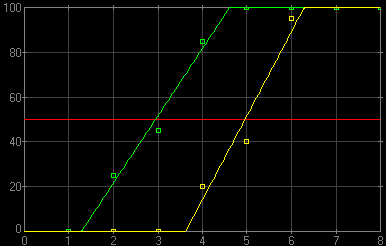
This no longer looks as nice as the lines from A quick and dirty approach now would be to drive straight lines through both colors of points "by eye" and then measure the horizontal distance between them at the 50% level. This would be, however, unscientific and unmanly; lets do it the right (or, at least, "righter" way). In this approach, I will be approximating the data points with the simplest model possible, where the success probability is 0 up to some EV value, v0, 100% above some v100 (higher), and a linear function of EV between these two. Computing the parameters v0 and v100 can be done with use of one of standard data reduction methods. For those familiar with statistical methods: I'm using here a best chi-square fit with two free parameters, and without statistical weights attached to the points. This is fairly primitive, but good enough for the purpose. A maximum likelihood fit based on the binomial distribution would be more proper (statistically more accurate and unbiased), but this would be really hairsplitting, in addition to more work. Then for each series (with and without IS, that is), v50, or the EV value corresponding to the 50% success rate, can be computed as (v0+v100)/2 the difference between these two values of v50 is our Δv50, done.
Here is how it looked in our simulated example. The linear model resulting from the fit is shown in colors as before; and the line parameters are:
|
| 
| Actually, I was lucky in this series. The mean square deviation from the model value of Δv50 for ten such simulation series using the same model was 0.04; I've checked that to get some idea about the statistical accuracy of the procedure which uses just 20 frames per data point. The only thing remaining now is to apply the same numerical procedure to the real data, so that we can, at long last, estimate our metrics for a real camera. Experiment design For that, however, we have to develop an experimental procedure to generate data points. The procedure should at least try to eliminate any statistical bias sneaking into the estimation process. Here is what I am using. A high-contrast target with lots of detail (my computer LCD screen) is photographed handheld from a distance of about one meter at shutter speeds progressing in 1 EV increments over a wide enough interval. (For longest focal lengths the distance may be larger; the point is to keep it the same for both series.) The shutter speed range has to be wide enough to include both extremes: v0 and v100 (0 and 100% success rate, respectively). For a wide angle (say, 28 mm EFL), a range from 1 s to 1/125 s should be just fine, while for longer lenses (300 mm EFL) you may have to go from 1/10 s to 1/1000 s or so. At a given focal length, for every shutter speed I shoot 20 frames. This number seems to be a reasonable minimum (see the previous section). This gives 200 to 300 frames per one focal length (depending on the shutter speed range necessary to capture the full variability). All shots within one focal length should be done under similar conditions, to minimize the impact of uncontrolled variables. I chose to do them seated, with elbows not supported; the chair staying in the same position. I also try to control my breath and keep all subjective factors as constant as possible (also between series). At a given shutter speed I do the series with and without IS, randomly deciding which goes first. The pictures are taken in manual exposure mode, metered before the first frame shot for a given focal length. The camera uses autofocus, and in all shots is aimed at the same point on the screen, containing enough of contrasty detail to focus on. Evaluation of images All image files for a given focal length are transferred to a computer and scrutinized for blur. The process is performed anonymously and in random frame order: when evaluating an image I do not know whether what shutter speed was used and whether the IS was on or off. Every frame is assigned one of three ratings, while viewed in full-scale, fill-screen mode:
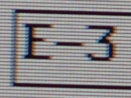
These are subjective evaluations, but this does not affect the results — as long as the same criteria are applied to images shot with IS as without, and as long as the evaluator does not know the control variables for a particular image. Statistical fluctuations will, obviously, affect the accuracy of results, but this will not introduce a systematic bias, and that's what counts. Instead of verbally describing my criteria for "good", "medium", and "bad", let me show you examples of each (F=150 mm) for one of the cameras submitted to this test, the Olympus E-3: | ||||
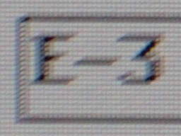 Subjective "bad" |
 Subjective "medium" |
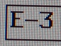 Subjective "good" |
|
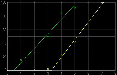
The LCD structure in the photographed text is quite helpful in detecting even a slight shake. The "bad" sample is, by the way, quite close to "medium", some are much worse. After tagging all frames this way, there is no more any reason to keep the process anonymous. Each IS/shutter point has its "goodness" value computed: percentage of "good" frames (with two "medium" counting as one "good"). This is used as the success rate in the procedure described under Benefit metrics estimation above. For example, a series of 10 "good" and 6 "medium" frames out of 20 will have a score of 65%: (10+6/2)/20. This is slightly different than dividing the results into "good" and "bad" only, but it does not affect the validity of using the half-height line offset as the IS benefit metrics. At the same time it reduces, I believe, fluctuations. The score-versus-EV points are then submitted to the numerical procedure as already described to come up with the Δv50 metrics. Example Here is an example of results obtained, again, for the Olympus E-3, with a zoom lens set to the focal length of 150 mm.
The line without IS (yellow) crosses the 50% level at v50=5.18, what is equivalent to the shutter speed of 1/36 s. We may say that this speed is 50% handholdable.
| With IS (green), v50=2.81, what corresponds to 1/7 s. The benefit of image stabilization, Δv50, can be then estimated at 2.37 EV, or a 5.2× factor in shutter speed.
| 
| So far I've used this method to estimate the IS benefits for four cameras: Olympus E-510 and E-3 SLRs, and the E-M1 (original and Mark II) of the OM-D series. I was also happy to see this method used by a number of photography Web sites. I would be even happier if the authors followed the good tradition of including a reference to the original source, but this is just a secondary issue of good manners, no harm done. | ||

|
Back to the Nitty-Gritty section, with articles on technical aspects of photography. |
| This page is not sponsored or endorsed by Olympus (or anyone else) and presents solely the views of the author. |
| Home: wrotniak.net | Search this site | Change font size |
| Posted 2009/02/28; last updated 2020/01/20 | Copyright © 2009-2020 by J. Andrzej Wrotniak |